Do We Really Need More Compute?
Scaling laws justified ever larger models. Yet frontier models use a sliver of themselves per token, and small specialists can beat giants at their own task.
›Contents
Imagine a laptop with 25 GB of RAM and twelve CPU cores starting a language model with 744 billion parameters.Just few moments later, the terminal prints a reply: "Ciao! Come posso aiutarti oggi?"
To be precise, the model alone would need about 1.5 TB of memory, so it shouldn't fit entirely on RAM. Yet, it runs because the laptop never holds it as a whole: most of the weights stay on the disk, and only a small part the model is loaded into the RAM for current tasks. It is slow, but it works.
The trick behind it, was explored in the project called colibrì (Italian for hummingbird), which exploits the fact that model LLM almost never use all of themselves at once.
Industry assumption so far has been that a better model requires a bigger model, and a bigger model requires more compute. This assumption is not wrong, and it is supported by some empirical results, yet it may be incomplete.
The question I want you to think about is:
Do we really need more compute, or do we need to use the compute we already have more intelligently?
The law that justified scale
In 2017, researchers at Baidu noticed a regularity in their experiments' results: the error of a neural network fell predictably as the training set grew, following a power law (Hestness et al., 2017).
Three years later, OpenAI turned that observation into a recipe for success. Kaplan et al. trained hundreds of language models and showed that the test loss falls as a power law in the number of parameters , the size of the dataset and the training compute , as long as none of the three becomes a bottleneck (Kaplan et al., 2020):
On a log-log plot these are straight lines, and they held over more than seven orders of magnitude. The suggested implication is that: performance could be bought. If you knew how much compute you could afford, you could forecast how good your model would be before training it. A few months later GPT-3 arrived with 175 billion parameters, more than ten times its predecessor, and indeed succeded (Brown et al., 2020).
In 2022, DeepMind modified this recipe, not the law. Most large models, according to them, were too big for the data they had seen. Modelling the loss as
where is the irreducible loss of language itself, since they found that parameters and training tokens should grow together, at roughly 20 tokens per parameter. Their 70B-parameter Chinchilla, trained on 1.4 trillion tokens, beat much larger model with the same amount of compute (Hoffmann et al., 2022).
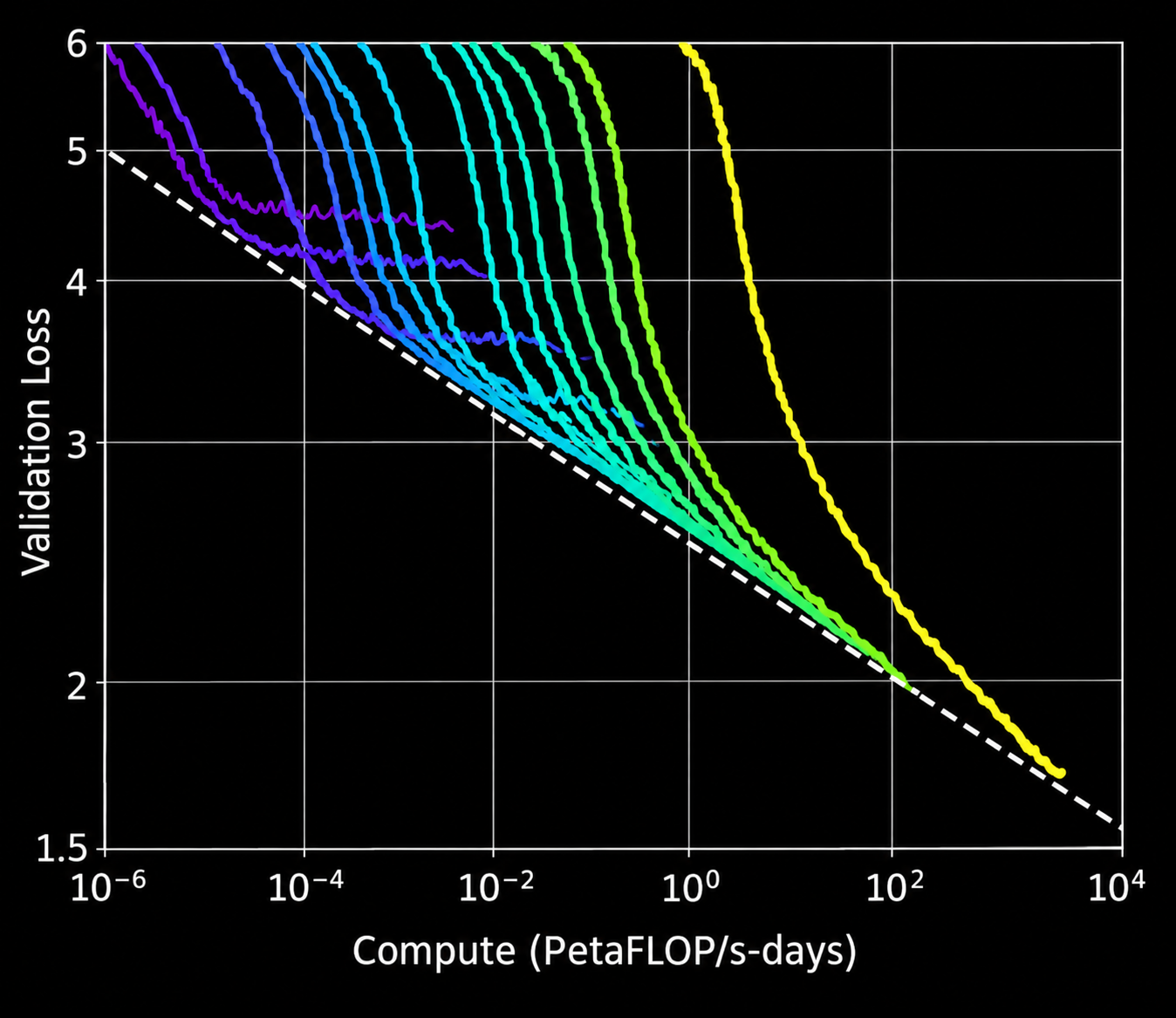
Nevertheless, this is not all, since the the equations also tell us that ten times more compute reduces the loss by only
Given this, the scaling law is therefore both the strongest argument for building larger models and a somewhat precise measure of how expensive that strategy becomes.
Most of the model sleeps
colibrì is an open-source engine written in C that runs very large open models on ordinary hardware (colibrì, 2026). Its reference model, GLM-5.2, has 744B parameters, but uses only about 40B of them for each token, about 5.4%. Moreover, only about 11 GB of weights actually change from one token to the next.
GLM-5.2 achieves this by using a mixture of experts (MoE), instead of a single feed-forward block. Every layer contains many smaller networks, the experts, and a learned router that sends each token to only a few of them (Shazeer et al., 2017; Fedus et al., 2022). For a token and experts , the layer computes
where are the router's scores and only the top experts are evaluated. The rest of the layer is not computed at all.
Therefore colibrì, make possible to dense part of the model (attention, shared experts and embeddings) to stay in RAM, while the routed experts stay on disk and are read only when the router asks for them. To address speed concern, a cache learns which experts the user's work requires, so the engine gets faster the more it is used. The developers even mapped where the specialists live: in GLM-5.2, 13,260 experts cluster into regions such as Python, SQL, mathematics, poetry and law, and routing is predictable enough that 71.6% of the next layer's choices can be anticipated one layer ahead.
This approach is not an exception, since every open top model is sparse:
| Model | Total parameters | Active per token | Share |
|---|---|---|---|
| DeepSeek-V4-Pro | 1.6T | 49B | ~3.1% |
| DeepSeek-V4-Flash | 284B | 13B | ~4.6% |
| GLM-5.2 | 744B | ~40B | ~5.4% |
| Qwen3.6-35B-A3B | 35B | 3B | ~8.6% |
The largest closed labs do not share publicly their architectures, therefore it is impossible to know with certainty, but usually even in dense Transformers, only a few percent of the neurons in a feed-forward layer are non-zero for any given input (Li et al., 2023).
Just as a quick reminder, the breadth of knowledge that a model has is measured, as proxy, by the Total number of parameters, while active parameters measure the cost of using it.
Your next question might be: what stops people from running these models locally then?. Well, today quite a lot!
colibrì decodes GLM-5.2 at 0.05–0.1 tokens per second on the laptop where the project started, and at about 1.8 tokens per second on a 128 GB workstation, so its is slow. Moreover, open models still follow the best closed ones, and a subscription often comes with tools and agents rather than only a model. Yet, these Hyperscaler are not profitable as of today, and their path to profitability is not clear, therefore if costs would start to rise then current market dynamics might shift user towards solutions such sa colibrì.
Small models, sharp tasks
Sparsity reduces the cost of a large model, nevertheless specialisation ask if after all one single model would't be better.
In October 2026, Mistral released Timestral, a family of time-series foundation models with 5M, 28M, 123M and 209M parameters (Mistral AI, 2026). The largest ranks first on the field's three main public benchmarks, GIFT-Eval, TIME and fev-bench, beating the previous state of the art model with only two-thirds of its parameters. The 28M model beats Chronos-2, a model which is about four times bigger.
To put this in perspective, the largest Timestral model is about 200 times smaller than the active part of GLM-5.2 alone, and almost 8,000 times smaller than the whole of DeepSeek-V4-Pro.
More importantly, Timestral does not need a GPU. On a standard server CPU with 8 threads, forecasting one day ahead from three weeks of 15-minute data takes 10 ms with the 5M model and 140 ms with the 209M model. The trade-off between size and accuracy is visible, but small: the 123M model comes within 0.2% of the best model performance at three-quarters of its latency.
The reason why it works is that a forecast is just a narrow task with a precise structure: trends, seasonality, noise and covariates such as calendars or weather. A model does not need to know poetry or corporate law to forecast a heat pump's vibration, and most of its training data can therefore be synthetic, fundamentally generated to contain exactly the pattern needed. On the other hand, a general LLM, if asked to forecast, would use billions of parameters that are irrelevant to the problem.
Interestingly, Mistral's showed an example, where they monitor thousands of industrial sensors continuously and, only when the model flags an anomaly, calls a LLM to investigate maintenance logs and manuals. A small specialist works all the time, while a large generalist is called upon only when needed. It is the logic of a mixture of experts, applied to an entire system.
Frontier quality, at a fraction of the price
DeepSeek released in April 2026 DeepSeek-V4-Pro, with 1.6 trillion parameters, of which only 49 billion are active per token, together with a sparse attention design that makes a context of one million tokens the default (DeepSeek, 2026).
This model is not the best available. On SWE-benchmarks its strongest configuration scores only 80.6%, against 88.6% for Claude Opus 4.8. However, its API costs are around $3.96 per million output tokens, roughly six times less than Opus.
The idea is not that DeepSeek beat the scaling law, but that by choosing what to compute, a lab can reach most of the frontier's quality for a fraction of the compute per token.
Conclusion
The scaling law is not broken. Larger models trained with more compute still perform better, and the hardest problems, such as the gap between DeepSeek and the best closed models, are still being solved by scale.
What has changed is how the compute is used. Frontier models activate a few percent of their parameters per token, small specialists can beat large generalist on specific tasks, and open models reach near-frontier quality at a fraction of the cost per token.
The answer to the initial question:
Do we really need more compute, or do we need to use the compute we already have more intelligently?
is therefore probably yes, but not everywhere. We need more compute to push the frontier, but not necessarily to use it. The next AI leap may come less from building a bigger brain than from learning which small part of it to wake up.
Useful Readings
- Vincenzo Fornaro, colibrì README and documentation (2026).
- Mistral AI, “Introducing Timestral” (2026).
- Cameron R. Wolfe, “Scaling Laws for LLMs: From GPT-3 to o3” (2025).
References
- Joel Hestness et al., “Deep Learning Scaling is Predictable, Empirically”, preprint (2017).
- Noam Shazeer et al., “Outrageously Large Neural Networks: The Sparsely-Gated Mixture-of-Experts Layer”, Proceedings of ICLR (2017).
- Jared Kaplan et al., “Scaling Laws for Neural Language Models”, preprint (2020).
- Tom B. Brown et al., “Language Models are Few-Shot Learners”, Advances in Neural Information Processing Systems (2020).
- Jordan Hoffmann et al., “Training Compute-Optimal Large Language Models”, Advances in Neural Information Processing Systems (2022).
- William Fedus, Barret Zoph and Noam Shazeer, “Switch Transformers: Scaling to Trillion Parameter Models with Simple and Efficient Sparsity”, Journal of Machine Learning Research (2022).
- Zonglin Li et al., “The Lazy Neuron Phenomenon: On Emergence of Activation Sparsity in Transformers”, Proceedings of ICLR (2023).
- DeepSeek, “DeepSeek V4 Preview Release” (2026).
- Mistral AI, “Introducing Timestral” (2026).
- Vincenzo Fornaro, colibrì: run frontier MoE models on hardware you already own (2026).