When the World Moves, the Prediction Should Follow
Equivariance in deep learning tells us how a neural network predictions should change when the input is transformed.
›Contents
Rotate a photograph of a dog and it remains a dog. Rotate its segmentation mask and the mask should rotate with it.
These two statements sound almost obvious, but the former ask the classifier to ignore the rotation, while the latter ask for its preservation in the output. The first property is called invariance, the second: equivariance.
Most neural networks are expected to learn these behaviours from examples. Show the model enough rotated dogs, translated molecules, or permuted point clouds and it may eventually infer which changes matter and which don't. This works, but it also mean spending data and more parameters on relearning structure that was already (the features of a rotated dogs stays the same).
Equivariant deep learning starts from the opposite position: if a transformation has a predictable effect on the task, then it should be encoded directly.
This article expands on a report I wrote about Equivariant Adaptation of Large Pretrained Models. The paper introduces EquiAdapt, a wrapper that makes a pretrained model equivariant by learning how to return each input to a canonical pose before prediction (Mondal et al., 2023). Its central finding is more general than the method itself: mathematical symmetry is useful only if it remains aligned with the distribution on which the model learned.
What should a neural network know before it sees any data?
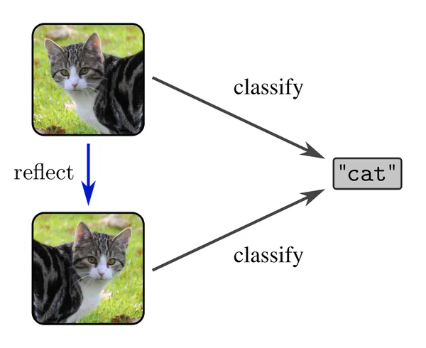
Invariance example.
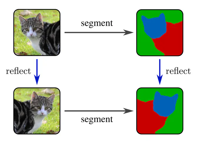
Equivariance example.
Symmetry as a transformation
A symmetry is not merely a visual resemblance, but it is a transformation under which some relevant structure is preserved.
The natural language for these transformations is a group. A group contains a set of elements and an operation satisfying four conditions:
- Closure: for all .
- Associativity: .
- Identity: there is an such that .
- Inverse: every has a satisfying .
The group describes how transformations compose. To describe what they do to data, we also need a group action. For a vector space , a linear action is represented by
where is the set of invertible linear maps on . A representation respects the group structure:
Obviously, the same abstract group can act differently on different spaces. A rotation may rearrange image pixels in the input, rotate a mask in the output, or multiply a feature vector by a representation matrix.
Some groups appear repeatedly in machine learning:
| Group | Transformation | Typical data |
|---|---|---|
| discrete planar rotations | Images with a finite set of orientations | |
| Discrete rotations and reflections | Images and regular polygons | |
| , | Continuous rotations in 2D or 3D | Images, molecules and point clouds |
| Rotations and translations in dimensions | Rigid-body systems | |
| Rotations, reflections and translations | Physical and geometric data | |
| Permutations of elements | Sets, graphs and particles |
The correct group is determined by the task, not by the data type alone.
Invariance and equivariance
Let be a model, with representations and acting on the input and output spaces. The model is -equivariant if
The equation says that transforming the input before applying the model is equivalent to applying the model first and then transforming its output; or, in other words the two operations commute.
The model is -invariant if
Invariance is therefore a special case of equivariance in which the output carries the trivial representation:
| Task | Desired transformation law |
|---|---|
| Image classification | Rotating the image should not change the class: invariant |
| Semantic segmentation | Rotating the image should rotate the pixel labels: equivariant |
| Object detection | The category stays fixed while the bounding box transforms: mixed |
| Molecular energy prediction | Rigid motion should not change a scalar energy: -invariant |
| Molecular force prediction | Rotations should rotate force vectors: -equivariant |
| Set classification | Reordering elements should not change the label: permutation-invariant |
| Node prediction on a graph | Reordering nodes should reorder node outputs: permutation-equivariant |
This distinction matters because throwing away a transformation too early can be convenient but also destructive. In particular, equivariance retains the transformation in a controlled way; invariance removes it.
Orbits, stabilizers and what the model sees
For an input , its orbit is the set of all versions reachable through the group:
An invariant model is constant across this orbit. An equivariant model is not constant, but its outputs across the orbit are completely determined by one prediction and the output action .
Some transformations may leave unchanged. They form the stabilizer
Stabilizers are often trivial for an asymmetric object in a "generic" pose, but not for instance for a circle, sphere, regular polygon, etc. (no matter how you rotate a sphere, it looks exactly the same, so every rotation in sits in its stabilizer). If is equivariant and , then
The output must preserve every symmetry of the input. In stabilizer notation,
This compact relation is the "neural-network version" of Curie's symmetry principle: a deterministic equivariant map cannot produce an output with less symmetry than its input. If a task requires one specific direction to be chosen from a perfectly symmetric object, the model needs extra information, randomness, or an explicit reference frame.
Why equivariance is useful
Equivariance is an inductive bias, meaning it restricts the functions a model is allowed to learn. That restriction can help in three ways.
-
First, it reduces sample complexity. If all rotated versions of a pattern must be processed consistently, the network does not need to learn each orientation. Parameters can be shared across the group orbit.
-
Second, it provides systematic generalization. Data augmentation encourages similar behaviour on transformed samples, but a mathematically equivariant architecture specifies such behaviour in its architecture.
-
Third, it can enforce physical consistency. For particles with positions , a scalar energy should satisfy while forces should satisfy
The coordinates frame is arbitrary, but physics is not. Encoding this distinction is particularly valuable in scientific machine learning, where a numerically plausible prediction can still violate a physical law or geometric constraint.
There is no universal benefit, however, since if a false symmetry is learned, then it produces a false constraint (a flipped 6 is a 9, yet is wrong invariance). Therefore, the important question is not whether a model should be equivariant, but to which group, at which layers, and for which outputs.
Four ways to learn a symmetry
Deep-learning systems usually obtain invariance or equivariance through augmentation, architectural design, group averaging, or canonicalization. These approaches encode the same prior with different guarantees and costs.
Data augmentation
For a loss , group augmentation optimizes an orbit-averaged objective such as
where is a distribution over transformations. This encourages the correct relation on sampled transformations, but it does not guarantee it. Moreover, the model can still behave inconsistently across training examples, and continuous groups have infinite augmented dataset.
Augmentation also changes the training distribution, which is harmless only when the augmented samples remain meaningful and aligned with the downstream task. For instance, training on 90-degree rotations of trains spends capacity on poses the model will almost never encounter while executing its tasks.
Architectural equivariance
An architecture can restrict every layer to commute with the group action. For a linear layer , equivariance requires the relation
Where the permissible weights lie in the solution space of these linear constraints.
Ordinary convolution is the familiar example. If translates a signal by and is a kernel, then
Convolution is therefore translation-equivariant. Group-equivariant CNNs replace translations with richer discrete groups, while steerable CNNs constrain kernels through group representations and irreducible components (Cohen and Welling, 2016; Weiler and Cesa, 2019). In three dimensions, Tensor Field Networks use spherical harmonics and representation coupling to obtain rotation and translation equivariance (Thomas et al., 2018).
This approach gives strong guarantees, but these specialized layers make existing architectures difficult to reuse. For a large pretrained backbone, this would likely mean traning a new model.
Group averaging
For a finite group and an arbitrary prediction model , the Reynolds operator constructs an invariant function
For equivariant outputs, each prediction must first be moved back into a common output frame:
This is the basis of frame averaging and Equi-Tuning. Under a squared-distance objective, the Reynolds operator can be seen as projecting a pretrained model onto the space of -equivariant functions (Puny et al., 2022; Basu et al., 2023).
The cost is direct: exact averaging requires backbone evaluations. Continuous groups require integration with respect to the Haar measure,
which is usually approximated by Monte Carlo samples. For a large backbone, this makes inference extremely costly and lengthy.
Learned canonicalization
Canonicalization on the other hand selects a representative pose from each orbit. Let be any prediction network and let
predict the transformation associated with an input. The canonical sample is
After prediction, an equivariant task restores the original output pose:
For an invariant task, is trivial and the final restoration disappears.
The construction becomes equivariant when the canonicalizer respects
Indeed, the inverse cancels the input transformation, while the output factor contributes . The main network itself does not need to be equivariant (Kaba et al., 2023).
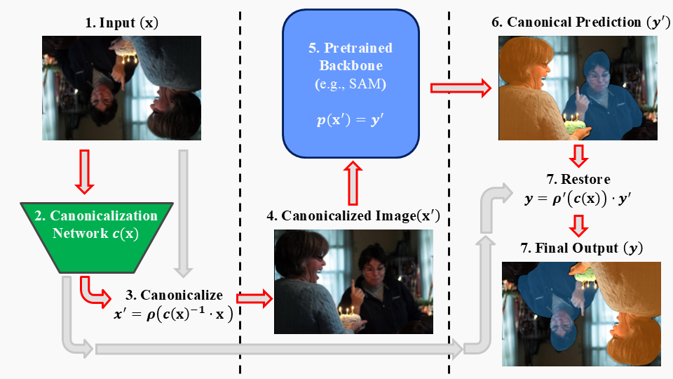
EquiAdapt model functioning.
The pretrained-model problem
Canonicalization appears to solve the architectural problem: attach a small network in front of a large pretrained backbone, transform the input into a canonical pose, and run the expensive model only once.
The difficulty is that an orbit has no inherently preferred "orientation/transformation". A canonicalizer may consistently rotate every upright image by , even if it makes no sense, such as upside down cars. This is mathematically valid, but a backbone pretrained mainly on upright cars images may perform badly on the resulting distribution.
Naive learned canonicalization creates two related problems:
- Alignment: the chosen canonical pose may not match the orientations preferred by the pretrained backbone.
- Augmentation: early in training, a random canonicalizer can expose the backbone to extreme transformations that are unnecessary for the task.
EquiAdapt addresses both with a canonicalization prior. Let denote the dataset's preferred distribution over and the distribution predicted by the canonicalizer. The regularizer is
If the prior density is fixed and the canonicalizer predicts , the entropy of the prior is constant. Minimizing the KL divergence is therefore equivalent to minimizing the cross-entropy
For a discrete group such as , an identity prior places all mass on :
The model is not being told to ignore rotations. It is being encouraged to map the training distribution back to the identity pose, so the backbone continues to receive inputs resembling those on which it was pretrained.
For continuous rotations, EquiAdapt uses an isotropic matrix Fisher distribution on :
where is the mode and controls concentration. With a prior centred at the identity, the orientation-dependent part of the loss becomes
where denotes equality up to an additive constant. The trace is largest when the predicted rotation is closest to the identity.
In practice, discrete canonicalizers can output one logit per group element, apply a softmax, and select with an argmax using a straight-through gradient estimator. Continuous canonicalizers must output valid rotation matrices, often by predicting vector fields and orthonormalizing them. That additional geometry makes continuous optimization much less forgiving.
What the experiments show
The most revealing result is not simply that prior-regularized learned canonicalization improves rotated accuracy. It is that it recovers robustness without giving up most of the original-distribution performance.
On CIFAR10, the following models were fine-tuned from ImageNet-pretrained and evaluated both on the original test set and on a test set averaged over the eight rotations in :
| Backbone | Method | Original accuracy ↑ | -average accuracy ↑ |
|---|---|---|---|
| ResNet50 | Vanilla | 96.97 ± 0.01 | 57.77 ± 0.25 |
| ResNet50 | Rotation augmentation | 94.91 ± 0.07 | 90.11 ± 0.19 |
| ResNet50 | Learned canonicalization | 93.29 ± 0.01 | 92.96 ± 0.09 |
| ResNet50 | augmentation | 95.76 ± 0.07 | 94.36 ± 0.09 |
| ResNet50 | Prior-regularized LC | 96.19 ± 0.01 | 95.31 ± 0.17 |
| ViT | Vanilla | 98.13 ± 0.04 | 63.59 ± 0.48 |
| ViT | Prior-regularized LC | 96.14 ± 0.14 | 95.08 ± 0.10 |
The vanilla models are accurate on familiar orientations and poor across the orbit. Naive canonicalization works but worse than prior-regularized one, which recovers much of the lost in-distribution accuracy while retaining transformation robustness (Mondal et al., 2023).
The canonical pose distribution supports the alignment explanation. On CIFAR10, the fraction of images mapped to the identity after training rose from 0.23 with naive learned canonicalization to 0.76 with prior regularization. The prior does not merely change the final classifier; it changes what the backbone is asked to see (Mondal et al., 2023).
The same trade-off appears in zero-shot instance segmentation on COCO:
| Backbone | Canonicalizer | Parameters | Original mAP ↑ | -average mAP ↑ |
|---|---|---|---|---|
| Mask R-CNN | None | 0 M | 45.57 | 27.67 |
| Mask R-CNN | Small G-CNN | 0.2 M | 35.77 | 35.77 |
| Mask R-CNN | G-WideResNet | 1.9 M | 44.51 | 44.50 |
| SAM | None | 0 M | 62.34 | 58.78 |
| SAM | Small G-CNN | 0.2 M | 59.28 | 59.28 |
| SAM | G-WideResNet | 1.9 M | 62.13 | 62.13 |
The equal original and rotated scores indicate near-perfect consistency, but it seems that the small canonicalizer becomes now the expressivity bottleneck, since increasing it from 0.2 million to 1.9 million parameters almost closes the Mask R-CNN gap. For SAM, the larger wrapper adds about 0.3% parameters and increases inference time by about 7.3%, far less than evaluating a 641-million-parameter backbone once per group element.
Point-cloud results show why this matters beyond images. Under arbitrary test rotations, a standard PointNet trained with only vertical-axis rotations falls from 85.9% to 19.6% ModelNet40 classification accuracy. Prior-regularized canonicalization with pretrained PointNet achieves 84.3 ± 1.2% without rotation augmentation. For DGCNN, the corresponding result is 90.2 ± 1.3%, compared with 33.8% for the conventionally trained model (Mondal et al., 2023).
Exact symmetry is not always available
Canonicalization has a structural ambiguity as seen before whenever we are dealing with a non-trivial stabilizer, since several group elements produce the same observed sample.
This motivates relaxed equivariance. Rather than requiring one exact transformation, the output may be correct up to the stabilizer coset:
The distinction is not cosmetic, because for a symmetric input, demanding a unique canonical direction can create discontinuities.
Continuous groups add further difficulties:
- Valid outputs must remain on a manifold such as rather than in unconstrained Euclidean space.
- Estimating or differentiating probability densities on the group can be expensive and numerically unstable.
- Monte Carlo group averaging introduces variance, while discretization replaces continuous symmetry with a finite approximation.
The original EquiAdapt experiments reported difficulty optimizing the continuous-rotation prior for images, even though the analogous construction was theoretically sounding and worked well for 3D point clouds.
Can canonicalization avoid equivariant networks?
EquiAdapt moves most equivariance constraints out of the backbone, but it does not make them disappear, we still need an equivariant canonicalizer, therefore this creates a circular-looking dependency, where to avoid a large equivariant architecture, we are obliged to build an additional equivariant network.
EquiOptAdapt reframes canonicalization as optimization over the orbit. Let be an ordinary, non-equivariant scoring network. Select the canonical transformation through
Every transformed input generates the same set of orbit scores, only re-indexed by the group action. If the minimum is unique, the selected group element changes predictably with the input; if it is not unique, the set of minimizers reflects the stabilizer.
The practical version learns embeddings for transformed inputs and converts them to a canonicalization distribution. With reference vector and temperature ,
An identity prior again aligns the chosen pose with the pretrained backbone:
The method learns canonical orientations with a non-equivariant scoring network and was reported to converge faster than EquiAdapt on the tested setting. Its evidence remains narrower, since the published experiments focus only on (Panigrahi and Mondal, 2024).
Measuring equivariance
Task accuracy does not measure equivariance, since a model can achieve similar average accuracy across rotations while producing inconsistent predictions for individual samples.
A direct normalized equivariance error is
where prevents division by zero. Exact equivariance gives up to numerical and interpolation error.
A serious evaluation should report at least three quantities:
- Task performance on the original distribution.
- Task performance across transformed or out-of-distribution samples.
- Equivariance error comparing the two computational paths directly.
Where equivariance matters most
Equivariance is most valuable when the transformation law is known independently of the dataset, meaning mostly in core scientific fields:
- Scientific machine learning: energies, forces, velocities and fields have precise behaviour under transformation, therefore -equivariant graph networks use these laws directly in message passing (Satorras et al., 2021)
- Robotics and perception: camera pose changes coordinates, not what we are seen, so predictions must remain consistent across viewpoints and reference frames
- Medical imaging: orientation and acquisition geometry may vary, while anatomical structures should transform predictably
- Point clouds and sets: the ordering of points is arbitrary, so making permutation invariance or equivariance is a basic requirement
- Pretrained-model adaptation: a small canonicalization module can add a missing symmetry without rebuilding an expensive backbone
Conclusion
Invariance means that a transformation should not affect the answer. Equivariance means that it should affect the answer in a known way.
That single distinction turns symmetry into a practical design principle. It explains weight sharing in convolutions, the consistency of geometric networks, and the possibility of adapting a large pretrained model without redesigning it. EquiAdapt also exposes the central complication: a mathematically valid coordinate system may still be the wrong one for the model behind it.
The goal is therefore not to make neural networks ignore geometry. It is to make their dependence on geometry explicit.
Useful Readings
- Sékou-Oumar Kaba et al., “Equivariance with Learned Canonicalization Functions” (2023).
- Arnab Kumar Mondal et al., “Equivariant Adaptation of Large Pretrained Models” (2023).
References
- Taco Cohen and Max Welling, “Group Equivariant Convolutional Networks”, Proceedings of ICML (2016).
- Nathaniel Thomas et al., “Tensor Field Networks: Rotation- and Translation-Equivariant Neural Networks for 3D Point Clouds”, preprint (2018).
- Maurice Weiler and Gabriele Cesa, “General E(2)-Equivariant Steerable CNNs”, Advances in Neural Information Processing Systems (2019).
- Omri Puny et al., “Frame Averaging for Invariant and Equivariant Network Design”, International Conference on Learning Representations (2022).
- Sourya Basu et al., “Equi-Tuning: Group Equivariant Fine-Tuning of Pretrained Models”, Proceedings of AAAI (2023).
- Siba Smarak Panigrahi and Arnab Kumar Mondal, “Improved Canonicalization for Model Agnostic Equivariance”, EquiVision Workshop at CVPR (2024).