A New Large Language Model
Diffusion language models replace next-token prediction with iterative denoising. The result is faster, more flexible generation, and a new set of trade-offs.
›Contents
Ask a conventional language model to write a sentence and it must make an initial commitment. It chooses the first token, then the second, then the third. Every decision becomes part of the context for the next one. Underneath it is still moving from left to right, token after token.
A diffusion language model work differently. It begins with a field of missing or corrupted tokens and repeatedly revises the whole field. Strangely, the middle may appear before the beginning; an uncertain word can remain masked while easier parts around it are settled. The model does not only choose what to write, but also where to write next.
For instance:
Step 0: [MASK] [MASK] [MASK] [MASK] [MASK] [MASK]
Step 1: [MASK] models [MASK] text [MASK] parallel
Step 2: Diffusion models generate text [MASK] parallel
Step 3: Diffusion models generate text in parallel
The idea is the same as behind my EDM-CSDI project. It learns to turn noise into plausible financial return sequences. Here, the same broad principle is applied to language: corrupt a sample of words, learn the reverse process, and generate by denoising.
Yet there is a key difference, while a return is a real number, so adding Gaussian noise has a natural meaning. A word is a discrete "symbol", therefore it lacks a obvious numerical path.
Diffusion language modelling begins with that problem.
Can a model generate language by revising an entire answer, rather than committing to it one token at a time?
Three ways to predict a missing word
Modern language models can be distinguished by what they are allowed to observe when predicting a token.
An autoregressive model generates from left to right. For a sequence , it factorizes the joint distribution as
This gives an exact and simple likelihood objective. Training can process all positions in parallel, but inference remains sequential because token must exist before can be sampled.
A masked language model, such as BERT, sees tokens on both sides of a randomly masked position and learns to reconstruct it. This produces strong bidirectional representations, but the original BERT objective was not designed as a complete procedure for open-ended generation (Devlin et al., 2019).
A masked diffusion language model turns masking into a full generative process. It trains across many corruption levels, starts generation from an entirely masked response, and progressively reconstructs the sequence.
| Property | Autoregressive LM | Masked LM | Masked diffusion LM |
|---|---|---|---|
| Context used | Tokens to the left | Visible tokens on both sides | Visible tokens anywhere |
| Generation order | Fixed, left to right | No native open-ended process | Flexible, iterative denoising |
| Tokens produced per pass | Usually one | Not applicable | Potentially many |
| Natural strengths | Fluent continuation, dynamic length | Representation and understanding | Infilling, editing, constrained and parallel generation |
| Main bottleneck | Sequential decoding | Not a general generator | Repeated full-sequence passes and dependency errors |
The distinction is therefore is more articulated than simply “GPT with random masks.” A diffusion model specifies a corruption process, a family of noisy intermediate distributions, and a learned reverse process that maps them back towards data, like it is done with images:
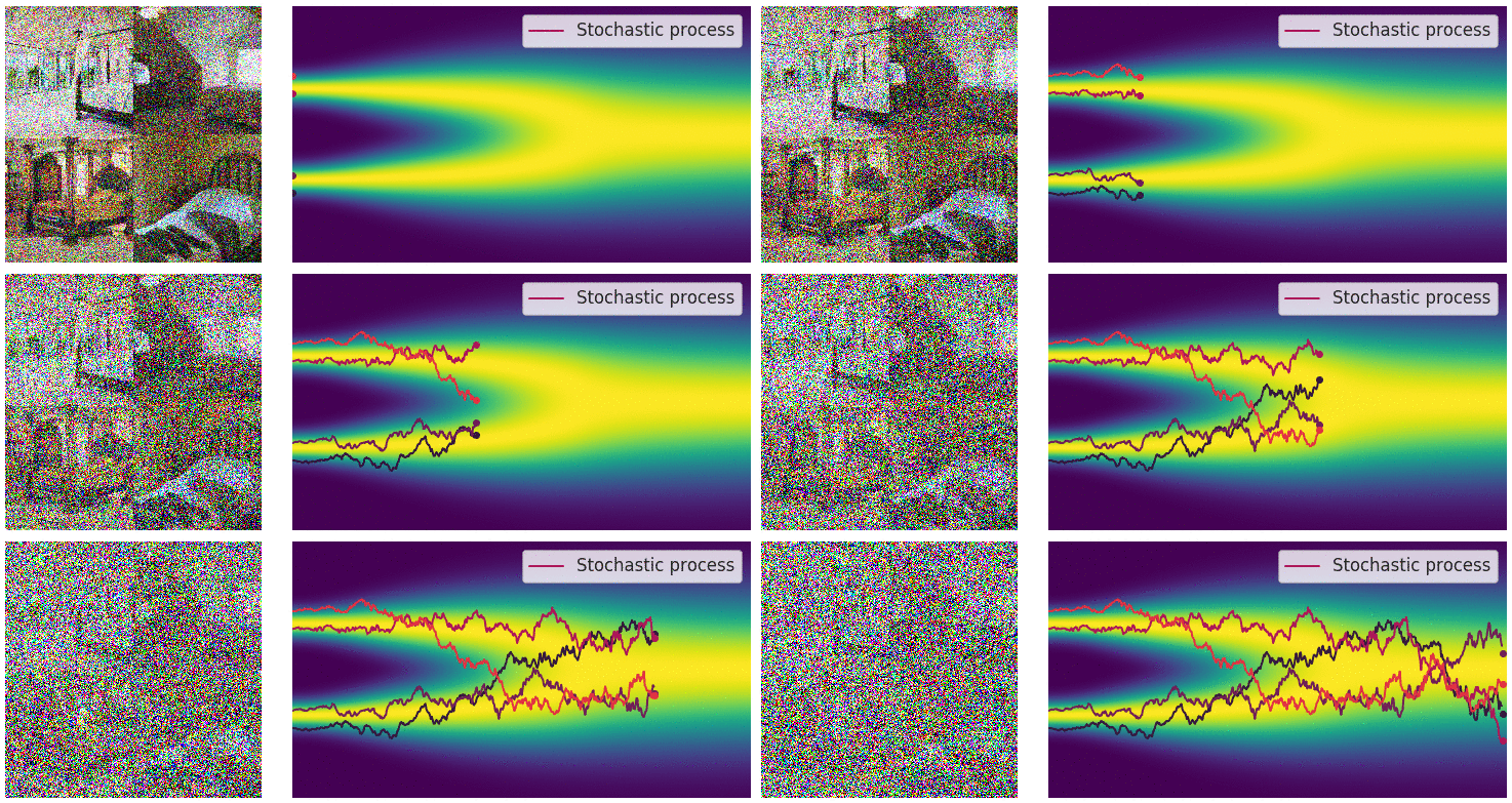
Forward process for Images, Source: Generative Modeling by Estimating Gradients of the Data Distribution, Yang Song.
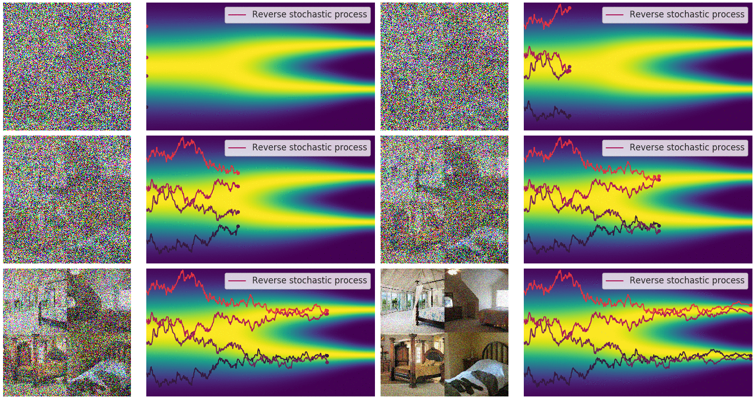
Reverse process for Images, Source: Generative Modeling by Estimating Gradients of the Data Distribution, Yang Song.
How discrete diffusion works
Let be the original token at position , a special [MASK] state, and the noise level. A common absorbing-mask process is
where and . Early in the process, most tokens remain visible. At , every position has been absorbed into the mask state.
The reverse model receives the corrupted sequence and predicts the clean token distribution at every masked position:
For masked diffusion models, the variational objective can be written as a weighted cross-entropy over masked positions:
The weight follows from the noise schedule. Under common parameterizations, this objective is a tractable variational upper bound on negative log-likelihood. D3PM first provided a general framework for diffusion over discrete state spaces, and later work simplified the masked objective and improved likelihood estimation (Austin et al., 2021; Sahoo et al., 2024).
Generation reverses the process:
- Keep the prompt fixed and initialize the response as masks
- Predict distributions for all currently masked positions using bidirectional attention
- Reveal a group of high-confidence tokens, while optionally remasking uncertain ones
- Repeat until the response is complete
The number of revealed tokens matters. Revealing many at once reduces latency, but their predictions are conditionally independent within that denoising step. Errors can therefore appear when two tokens need to be coordinated. On the other hand, revealing one token at a time protects coherence, but gives up much of the promised parallelism.
Continuous and discrete language diffusion
The first major approach, Diffusion-LM, mapped tokens into continuous embeddings and added Gaussian noise there (Li et al., 2022). If is the embedding sequence, the forward marginal resembles image and time-series diffusion:
A neural network denoises , after which the final vectors must be rounded or decoded back into vocabulary items. This makes classifier guidance and smooth latent manipulation possible, but creates a problem: Euclidean distance between embeddings does not necessarily correspond to any meaningful corruption path linguistically speaking.
Discrete diffusion stays inside token space. A transition matrix determines whether a token remains unchanged, becomes a random vocabulary item, or moves into an absorbing mask state:
Score Entropy Discrete Diffusion, or SEDD, instead learns ratios between probabilities of nearby discrete states and derives the likelihood bound for continuous-time Markov chains (Lou et al., 2024). Masked Diffusion Language Models, or MDLMs, show that the absorbing-mask have the advantage of simplifying the objective due to lower variance (Sahoo et al., 2024).
What the performance results actually show
While there is not a single leaderboard for autoregressive and diffusion language models together, because of different parameter counts, tokenizers, training data, post-training, sampling steps, etc., there are some useful evidence nevertheless.
Likelihood: closing the gap
On the One Billion Word benchmark, MDLM substantially improved over earlier diffusion methods. The following results show the 110M-parameter models trained under the protocols reported by Sahoo et al.:
| Training tokens | Model | Paradigm | Test perplexity ↓ |
|---|---|---|---|
| 33B | Transformer | Autoregressive | 22.32 |
| 33B | SEDD | Discrete diffusion | ≤ 32.79 |
| 33B | MDLM | Masked diffusion | ≤ 27.04 |
| 327B | Transformer | Autoregressive | 20.86 |
| 327B | MDLM | Masked diffusion | ≤ 23.00 |
Where perplexity is the exponential of average negative log-likelihood, so lower is better. The difference between autoregressive and diffusion stems from the fact that the former use exact likelihood while the latter only the upper bound. The table shows that masked diffusion is fairly close to autoregressive at large scale, even if it does not say anything about whether the two systems are equally efficient to train or sample (Sahoo et al., 2024).
Capability: competitive, but not better
LLaDA-8B showed that a diffusion language model trained from scratch on 2.3 trillion tokens could become competitive with Llama 3 8B on several in-context learning tasks (Nie et al., 2025). Dream-7B, initialized from Qwen2.5-7B and then converted to diffusion training reported unusually strong results on constraint-heavy planning: 81.0 on Sudoku, against 21.0 for Qwen2.5-7B. This seem to be consistent with the fact that bidirectional revision helps when later constraints should alter earlier choices (Ye et al., 2025).
These are not clear proofs of a better architecture, since Dream inherits knowledge from Qwen, the models saw different amounts of training data, and benchmark scores depend on decoding settings. A 2026 evaluation of eight masked diffusion models across 58 benchmarks found that they still lagged behind autoregressive models overall, with the lost of inter-token dependence as the main weakness of aggressive parallel prediction (Zhong et al., 2026).
Speed: the real advantage
DiffusionGemma provides one of the clearest comparisons because the diffusion and autoregressive modes share the same Gemma 4 foundation. Its text-diffusion mode refines blocks of 256 tokens and uses about 12 denoising steps on average.
| Metric | DiffusionGemma, diffusion | Gemma 4, AR + multi-token prediction |
|---|---|---|
| Output speed on one H100 | 1,479 tok/s | 303 tok/s |
| Tokens per forward pass | 19.74 | 1.40 |
| GPQA Diamond | 73.2 | 82.3 |
| LiveCodeBench v6 | 69.1 | 77.1 |
| HumanEval | 94.5 | 98.8 |
| IFEval | 97.4 | 98.7 |
The diffusion mode was approximately 4.9 times faster in this batch-size-one, excluding prompt prefill, but it was also weaker on most quality metrics (DiffusionGemma Team, 2026).
A diffusion model can be faster when it finalizes many tokens per pass, but if quality requires nearly one token per pass, the advantage largely disappears.
Where diffusion may matter the most
The strongest use case may not be ordinary chat, since autoregressive models are already highly optimized for open-ended and different length conversation. Diffusion becomes more attractive when the output has structure that can be solved globally.
-
Code and editing: the model can fill several related regions, revise definitions and satisfy constraints across a file
-
Infilling: text before and after a gap can be treated as an evidence without the need for any workaround for left-to-right
-
Planning under mutual constraints: Sudoku, schedules and layouts can benefit when a choice near the end reconstruction process should revise a choice near the beginning.
-
Fast low-concurrency serving: diffusion language models can be especially fast when the system is processing only one or a few users’ requests simultaneously.
Therefore, the broader technological direction may be hybrid, where block of diffusion generates groups of tokens autoregressively across blocks and diffusively inside each block, finding the right balance between strong sequential dependence and parallel decoding (Arriola et al., 2025). Moreover, the useful question may not be which paradigm "wins", but how much sequential structure a task actually requires.
The unresolved problems
Diffusion language models are credible alternatives, but still have several limitations:
-
Parallel predictions can conflict Tokens sampled together do not directly condition on one another, thus more parallelism can reduce syntax correctness and coherence
-
Length is awkward Many systems denoise a fixed "canvas" and must choose its size in advance
-
Full-sequence attention is expensive While autoregressive models reuse cached keys and values efficiently, diffusion models repeatedly revisit a changing sequence, making caching harder
-
Quality and speed are coupled More denoising steps allow correction but increase latency, and some parallel systems recover quality only at nearly token-wise decoding
-
The evidence is still little Many leading results are technical reports or preprint, and the largest autoregressive systems remain the most favorite choice for deployment
Conclusion
Diffusion language models generate text by gradually refining an entire response rather than writing one token at a time. This allows faster and more flexible generation, especially for tasks such as infilling, code editing and planning.
However, they are not yet a clear replacement for autoregressive models. Their speed can reduce coherence, while training, caching and variable-length generation remain difficult.
The question is therefore not which approach will replace the other, but when parallel revision is more useful than sequential generation.
Useful Readings
- Tianyi Li et al., “A Survey on Diffusion Language Models” (2025).
- Shen Nie et al., LLaDA project page (2025).
- DiffusionGemma Team, “DiffusionGemma Technical Report” (2026).
References
- Jacob Austin et al., “Structured Denoising Diffusion Models in Discrete State-Spaces”, Advances in Neural Information Processing Systems (2021).
- Xiang Lisa Li et al., “Diffusion-LM Improves Controllable Text Generation”, Advances in Neural Information Processing Systems (2022).
- Aaron Lou, Chenlin Meng and Stefano Ermon, “Discrete Diffusion Modeling by Estimating the Ratios of the Data Distribution”, Proceedings of ICML (2024).
- Subham Sekhar Sahoo et al., “Simple and Effective Masked Diffusion Language Models”, Advances in Neural Information Processing Systems (2024).
- Shen Nie et al., “Large Language Diffusion Models”, preprint (2025).
- Jiasheng Ye et al., “Dream 7B: Diffusion Large Language Models”, preprint (2025).
- Marianne Arriola et al., “Block Diffusion: Interpolating Between Autoregressive and Diffusion Language Models”, preprint (2025).
- Yangyang Zhong et al., “Parallelism and Generation Order in Masked Diffusion Language Models: Limits Today, Potential Tomorrow”, preprint (2026).