Conditional Latent Diffusion with SDEs
Conditional face generation with continuous-time SDEs, latent diffusion, and classifier-free guidance.
›Contents
Overview
Generating an image from noise is only half of the problem. The harder question is whether the generation process can be controlled without training a separate classifier for every desired attribute.
For the Hands-on Generative AI course at the Technical University of Munich, Marco Zimmatore and I built a conditional latent diffusion model from scratch. The project combines the continuous-time score-based framework introduced by Song et al. with a pretrained Variational Autoencoder and Classifier-Free Guidance (CFG).
The model trained by us on limited resources generates faces from the CelebA dataset while conditioning the reverse diffusion process on attributes such as age, expression, hair, and facial features. Rather than diffusing full-resolution images, it learns the score of their compressed latent representations.
The project compared:
- Variance Preserving (VP), Variance Exploding (VE), and subVP SDEs;
- Standard score matching, Likelihood Weighting (LW), and LW with Importance Sampling (LW + IS);
- CFG scales from 1.5 to 7.5;
- generative quality through FID, Inception Score, and latent-space NLL.
The best FID was 55.55 with VP and LW + IS, nearly identical to the VP baseline. Increasing the CFG scale strengthened the requested attributes, but progressively damaged perceptual fidelity: for the subVP baseline, IS rose from 3.23 to 4.09, while FID deteriorated from 58.38 to 77.86.
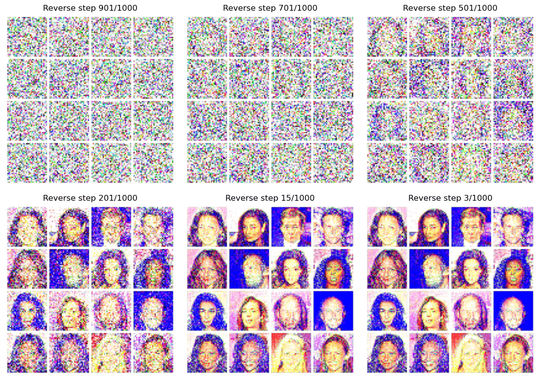
Reverse diffusion sampling for VP with Likelihood Weighting + Importance Sampling in latent space.
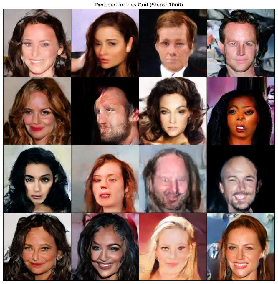
. Decoded output shown as a fixed reference.
The problem
Score-based diffusion models learn to reverse a process that gradually destroys the structure of the data. In pixel space, however, the network must model every visual detail at every diffusion step, making training expensive.
The project asked three related questions:
Can a compact latent diffusion model reproduce the continuous-time SDE framework, generate faces conditionally through CFG, and remain effective under limited computational resources?
Moving the process into latent space reduces the dimensionality of the learning problem, but it also creates a new dependency: the diffusion model must generate latents that remain compatible with a separately trained decoder.
This tension between computational efficiency and decoder compatibility represents one of the main findings of our project.
From images to latent diffusion
We used the pretrained stabilityai/sd-vae-ft-mse VAE to map an image into a lower-dimensional latent representation :
The diffusion process operates on , not directly on the image. After sampling, the VAE decoder maps the denoised latent back into pixel space:
| Component | Role |
|---|---|
| Pretrained VAE | Compresses CelebA images and decodes generated latents |
| Continuous-time SDE | Defines how latent representations are progressively noised |
| Conditional U-Net | Estimates the time-dependent score, or equivalently the added noise |
| Classifier-Free Guidance | Controls generation using CelebA attribute labels without a separate classifier |
| Euler-Maruyama solver | Numerically integrates the reverse-time SDE |
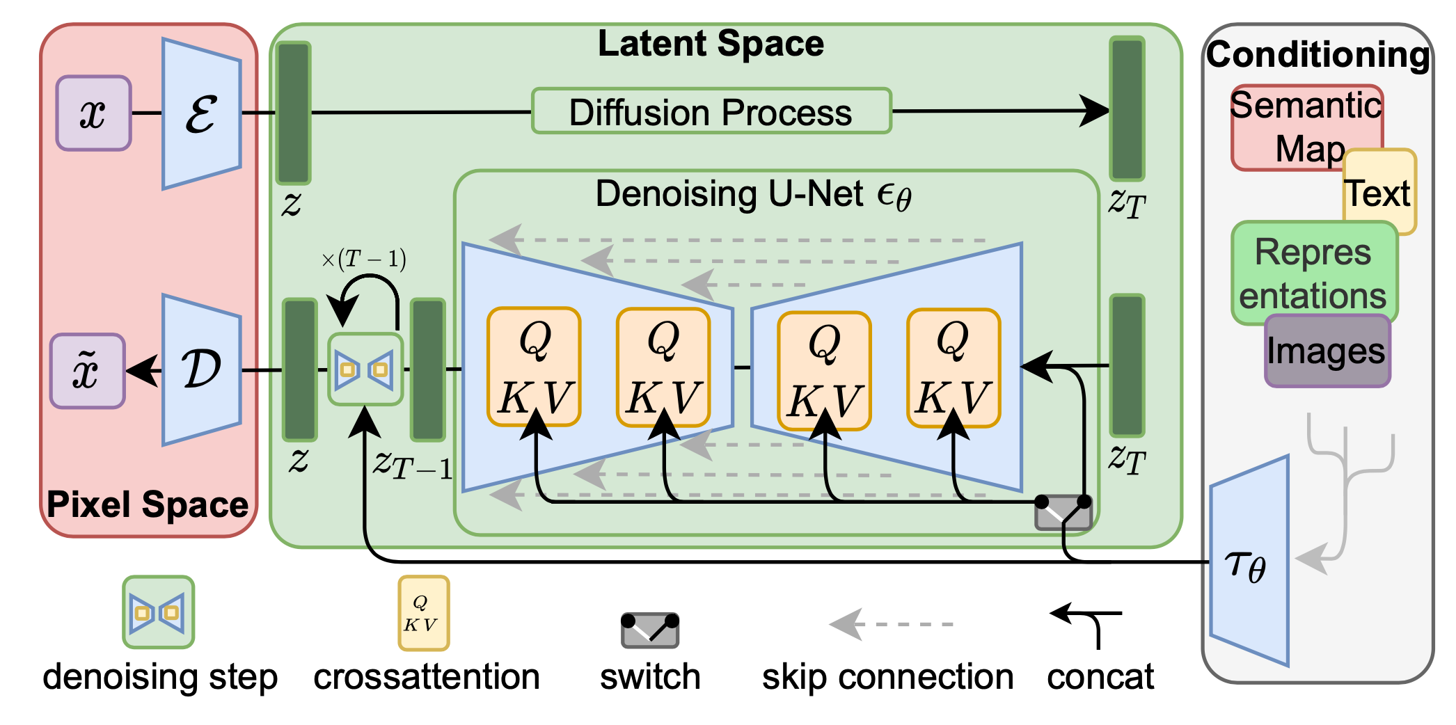
The architecture of the latent diffusion model (LDM). Source: Rombach et al., "High-Resolution Image Synthesis with Latent Diffusion Models," 2021.
The SDE formulation
Following Song et al., the forward diffusion process is written as an Itô SDE:
where is the drift, controls the injected noise, and is a standard Wiener process. At , follows the latent data distribution; by , it approaches a tractable prior such as .
Generation relies on the reverse-time SDE:
The unknown score is approximated by the U-Net . With a Gaussian perturbation kernel,
score estimation can be implemented as noise prediction:
We implemented three continuous-time processes:
| SDE | Main property | Observed behaviour |
|---|---|---|
| VP | Variance remains bounded throughout diffusion | Best overall FID and stable training |
| subVP | Reduced diffusion variance relative to VP | Competitive results and strongest response to CFG |
| VE | Noise variance grows without a drift term | Highest expressivity in theory, but slowest convergence in our constrained setup |
Conditional generation with CFG
During training, the attribute vector is randomly replaced with a null condition . The same network therefore learns both the conditional and unconditional scores.
At inference, the two estimates are combined as:
where is the guidance scale. The difference between the conditional and unconditional scores points sampling toward latents associated with the requested attributes.
The conditioning vector and the continuous diffusion time are embedded separately, combined through an MLP, and injected into the U-Net residual blocks using Feature-wise Linear Modulation:
This allows the same denoising network to adapt both to the current noise level and to the requested facial characteristics.
Architecture and training
The score network is a symmetric encoder-decoder U-Net built from residual blocks, learned downsampling, nearest-neighbour upsampling, skip connections, and self-attention at the lowest spatial resolutions.
| Setting | Value |
|---|---|
| Dataset | CelebA |
| Training images | Approximately 60,000 |
| Training iterations | Approximately 200,000 |
| Batch size | 16 |
| U-Net parameters | Approximately 12.9 million |
| Reverse sampling steps | 1,000 |
| Generated samples for FID and IS | 10,000 |
| Held-out latents for NLL | 1,000 |
Group Normalization was used instead of Batch Normalization because GPU memory constraints required small batches. Self-attention was restricted to the deepest feature maps, where global context is useful and the quadratic attention cost is lower.
The project was implemented as a modular PyTorch Lightning pipeline with YAML experiment configurations and Weights & Biases tracking. Separate modules handle the U-Net, SDE definitions, forward and reverse processes, VAE interface, training, and evaluation.
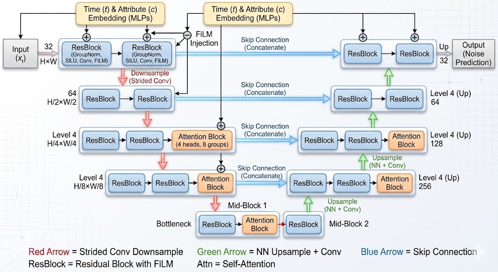
Architectural Overview of the Conditional U-Net.
Results across SDEs and objectives
FID and IS were calculated from 10,000 decoded samples. NLL was estimated on 1,000 held-out images through the probability-flow ODE, using the Hutchinson trace estimator.
Because the VAE was fixed, the reported NLL measures only the latent prior-matching term, not the full pixel-space reconstruction likelihood. It should therefore be interpreted within this project rather than compared directly with pixel-space benchmarks.
| SDE | Objective | Guidance | FID ↓ | IS ↑ | Latent NLL ↓ |
|---|---|---|---|---|---|
| subVP | Base | 1.5 | 58.38 | 3.23 | |
| subVP | LW | 1.5 | 67.16 | 3.11 | |
| subVP | LW + IS | 1.5 | 56.70 | 2.86 | |
| VP | Base | 1.5 | 55.56 | 2.90 | |
| VP | LW + IS | 1.5 | 55.55 | 2.90 | |
| VP | LW | 1.5 | 69.59 | 3.00 | |
| VE | Base | 1.5 | 77.32 | 3.09 |
Three results stand out:
- VP produced the best perceptual fidelity. Its baseline and LW + IS variants were effectively tied on FID.
- Likelihood Weighting alone consistently degraded FID. In latent space, emphasizing all noise levels may force the model to spend capacity on high-frequency artifacts inherited from the fixed VAE.
- VE underperformed despite its theoretical expressivity. Its slower convergence was a poor match for the available training budget.
Denoising process with 1000 reverse steps for VP trained with LW + IS and 1.5 guidance (left), subVP trained with LW + IS and 1.5 guidance (center), and VE with 1.5 guidance (right). Reconstruction started from N (0, I) for VP and subVP, and N (0, = 50.0) for VE
The guidance trade-off
Changing only the CFG scale produced a clear and monotonic trade-off for the subVP baseline:
| Guidance scale | FID ↓ | IS ↑ |
|---|---|---|
| 1.5 | 58.38 | 3.23 |
| 3.5 | 62.16 | 3.54 |
| 5.0 | 67.34 | 3.78 |
| 7.5 | 77.86 | 4.09 |
Higher guidance made attributes more distinct, which increased IS. At the same time, FID worsened at every step, indicating that generated images moved further from the real CelebA distribution.
This is not a contradiction between the metrics. IS rewards recognizable and diverse class features, while FID penalizes a shift in the overall generated distribution. Strong guidance can improve the first while damaging the second.
Latent-decoder misalignment
One significant limitation was not simply insufficient training time. It came from separating the latent generator from the fixed VAE decoder.
Let the VAE aggregated posterior be
The decoder is trained primarily on latents from high-density regions of . The diffusion model, however, samples from an approximation . A latent can be plausible under the learned diffusion geometry while still lying outside the region on which the decoder learned a reliable inverse mapping.
Strong CFG may makes this failure mode more likely, since guidance extrapolates the conditional score field, large values of could push the trajectory into extreme conditional regions. When these latents are decoded, the result may contain distorted structure, incorrect colours, washed-out textures, or other artifacts.
This explains why the model could show a stronger conditional signal while receiving a worse FID score. The issue was not only what the diffusion prior learned, but whether the fixed decoder could interpret the latents it generated.
Limitations
The results should be read in the context of a course project with constrained compute.
- Training used approximately 60,000 CelebA images, a batch size of 16, and around 200,000 iterations
- The VAE was pretrained and fixed, preventing the encoder, decoder, and diffusion prior from adapting jointly
- Euler-Maruyama required 1,000 reverse steps, making generation slow and allowing numerical error to accumulate
- FID and IS do not directly measure whether every requested attribute is respected
- The latent NLL excludes the VAE reconstruction term and is not directly comparable with full image-space likelihoods
- Results from Song et al. use different data, architectures, and pixel-space training, so they provide context rather than a controlled benchmark
The most direct extensions would be to train or fine-tune the autoencoder jointly, evaluate explicit attribute accuracy, use higher-order samplers, test larger training budgets, and regularize guided sampling toward the typical latent region.
Conclusion
This project reproduced the core techniques and tools of score-based diffusion in latent space: continuous-time SDEs, a conditional U-Net, numerical reverse diffusion, and classifier-free guidance.
It identifies also how, with constrained training set up conditioning, CFG, and VAEs can influence the reconstruction process and its outputs.